Part-2: How to Design an ML System for ETA Prediction in Ride-Hailing Services
#18 Building the Solution – Model Selection, Training Strategies, and Deployment Pipeline
In Part 1, we established a solid foundation by carefully framing the problem, identifying impactful features, and performing essential feature engineering for ETA prediction. We asked critical questions to align our ML system with business requirements and technical constraints, and defined ETA prediction as a supervised regression task. If you missed it, you can catch up on Part 1 here.
In this Part 2, we'll focus on the next critical steps: selecting the right ML model, designing training strategies, evaluating the model effectively, and establishing a reliable deployment pipeline.

Model Selection: Choosing the Right ML Approach
Selecting an appropriate model for ETA prediction is crucial for balancing accuracy, inference speed, and scalability. Considering the complexity and real-time nature of ride-hailing ETA predictions, traditional models like Gradient Boosted Decision Trees (GBDT) and Factorization Machines (FM) show clear limitations. GBDT models typically struggle with handling large feature sets efficiently, while FM heavily depends on manually engineered feature representations, limiting its ability to capture complex, real-world interactions.
Given the vast scale and dynamic nature of traffic data, two promising options emerge:
Option 1: XGBoost (Optimized Gradient Boosted Trees)
XGBoost is highly effective for structured tabular data, offering rapid inference and interpretability. It naturally handles non-linear relationships among features (such as road type and traffic conditions) and efficiently manages high-dimensional data with minimal computational overhead. Its interpretability is advantageous, providing clear insights through feature importance metrics. However, its lack of sequential learning capabilities can limit its effectiveness in modeling rapidly changing traffic scenarios over extended routes.
Option 2: Wide-Deep-Recurrent (WDR) Learning Model
The WDR model combines linear components ("wide") for memorizing common routes, deep neural networks for capturing complex interactions among features, and recurrent architectures (like LSTMs or Transformers) for modeling sequential traffic patterns. This hybrid structure makes it powerful at adapting to real-time changes and sequential traffic patterns. However, WDR requires more significant computational resources, often GPUs, for training and inference, and poses challenges in interpretability.
Recommended Hybrid Approach
A practical solution is combining the strengths of both models:
XGBoost for initial fast predictions to meet real-time latency constraints.
WDR for refining predictions, especially for longer trips with significant changes in traffic conditions.
For example, a rider traveling from JFK Airport to Times Square might receive an initial prediction of 30 minutes from XGBoost, quickly adjusted to 32 minutes by the WDR model accounting for recent congestion near specific route segments.
Constructing Dataset
Creating the right dataset involves thoughtful handling of data splitting, feature engineering, and addressing key challenges.
Challenges & Trade-offs:
Data Sparsity: Real-time traffic data might be limited on less frequently traveled roads, leading to sparse or missing values. Employ robust handling mechanisms like imputation or embedding-based approaches.
Temporal shifts: Traffic patterns change over time due to events, weather, or infrastructure changes. Regular retraining or adaptive learning strategies help manage drift effectively.
Geographical diversity: Data distribution varies significantly across regions. Training on a diverse geographical dataset or fine-tuning models per region ensures scalability and robustness.
Data Quality & Noise: GPS inaccuracies and inconsistent reporting can introduce noise. Robust preprocessing and filtering mechanisms are essential.
Data Splitting:
Use a hybrid approach combining time-based and geographic splits to test model robustness. Train on historical data, validate on recent periods, and test on unseen, future data to mimic real-world scenarios.
Challenges & Trade-offs:
Balancing training set size with computational constraints.
Ensuring representativeness of validation/test sets across diverse cities and scenarios.
Frequent updates versus computational cost of retraining.
Having selected the model and dataset construction strategy, the next steps involve defining appropriate loss functions, training methodologies, evaluating the model rigorously, and building a reliable serving pipeline.
Loss Function
Selecting an appropriate loss function is essential:
Mean Absolute Error (MAE): Robust to outliers, suitable for ETA accuracy.
Mean Squared Error (MSE): Penalizes large errors heavily, useful if large deviations must be avoided.
Huber Loss: Balances between MAE and MSE, robust to outliers.
For ETA prediction, Huber Loss is typically preferred due to its robustness and balanced sensitivity.
Model Training Strategies
Model training strategies are methodologies or systematic approaches used to teach machine learning models by exposing them to relevant historical data. These strategies directly influence how effectively a model learns and adapts to data patterns.
Batch Training: A traditional training strategy where the entire historical dataset is processed together in batches. This method helps the model learn comprehensive patterns from past data and is commonly used when computational resources are stable and abundant.
Online Training: A continuous learning process where the model updates incrementally with each new data point. Ideal for rapidly changing environments, online training helps the model quickly adapt to real-time data streams, adjusting predictions to reflect the latest trends in data.
Transfer Learning: A method where models trained on extensive data from one context (e.g., one city) are fine-tuned or adapted to related but different environments (e.g., a new city). This strategy significantly reduces training time and resource demands by leveraging previously learned patterns.
Challenges & Trade-offs:
Batch training offers stability but lacks responsiveness to immediate changes.
Online training adapts quickly but may introduce instability or drift without proper regularization.
Transfer learning depends heavily on the relevance of source data to new scenarios.
Evaluation: Offline and Online Metrics
Proper evaluation metrics help measure model effectiveness and inform iterative improvements.
Offline Metrics
Offline metrics evaluate the model's performance using historical or pre-recorded data.
Mean Absolute Error (MAE): Measures the average magnitude of errors between predicted and actual values without considering direction.
Example: If ETA prediction errors are 1 min, 2 min, and 3 min, MAE = (1+2+3)/3 = 2 mins.
Root Mean Squared Error (RMSE): Measures the square root of the average squared differences between predicted and actual values, emphasizing larger errors.
Example: If ETA prediction errors are 1 min, 2 min, and 3 min, RMSE = sqrt((1²+2²+3²)/3) ≈ 2.16 mins.
Mean Absolute Percentage Error (MAPE): Expresses prediction accuracy as a percentage, useful for comparative analysis across different scales.
Example: If actual ETA is 30 mins and predicted ETA is 33 mins, the MAPE = |33-30|/30 × 100% = 10%.
Online Metrics
Online metrics assess real-time performance and user experiences directly in a live production environment.
Real-Time Accuracy: Tracks how close predictions are to actual arrival times in live settings.
Example: Real-time monitoring of predictions vs. actual arrival times across thousands of trips.
Latency: Measures the response time of the prediction system, ensuring predictions are delivered promptly.
Example: The average time taken by the model to generate predictions is measured to ensure it remains under 100 milliseconds.
User Satisfaction Metrics: Captures direct feedback from users regarding prediction accuracy and their overall ride experience.
Example: User ratings, complaints, or cancellations linked directly to ETA inaccuracies.
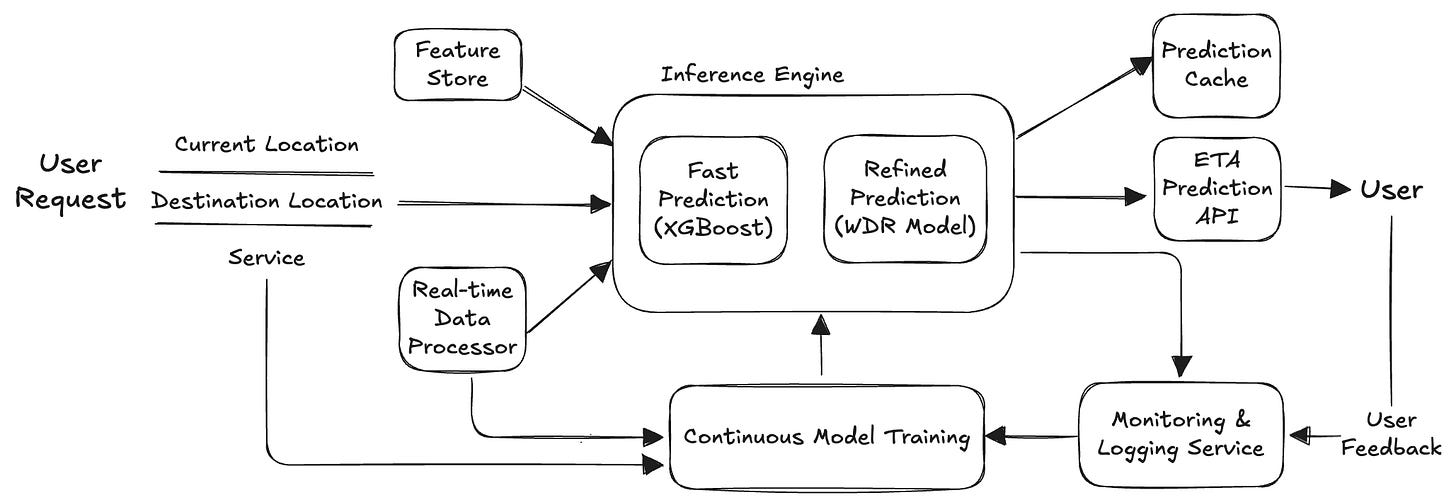
ML Model Serving Pipeline

A robust and efficient serving pipeline ensures that ETA predictions reach users quickly and reliably. Here’s a detailed breakdown of each component:
User Request: Users input their current location and desired destination, initiating the ETA prediction request.
Real-Time Data Processor: This component ingests and preprocesses real-time data, including traffic updates, GPS data, and contextual information like user location and recent activities. It transforms raw inputs into structured, model-ready features such as geohashes, real-time speed estimates, and cyclical encodings for time-related features.
Feature Store: Stores preprocessed features such as spatial geohash encodings, cyclical time features, and embeddings of categorical variables (e.g., driver profiles, road segments). The feature store allows fast retrieval and integration of these features at inference time.
Inference Engine: Consists of two complementary models:
XGBoost Model: Quickly generates baseline predictions using structured data, ensuring low latency.
WDR Model: Refines predictions dynamically, capturing more nuanced and sequential traffic conditions for improved accuracy.
Prediction Cache: Caches predictions for popular routes, serving these directly to users without repeated inference computations. This reduces latency significantly for frequently traveled routes.
ETA Prediction API: Exposes the final predictions via an API endpoint, ensuring predictions are promptly delivered to the user’s app.
Monitoring & Logging Service: Continuously monitors prediction accuracy, system latency, and user feedback, logging all relevant information for analysis. This helps quickly identify anomalies and ensures high-quality predictions are maintained.
Continuous Model Training: Incorporates real-time data collected from the monitoring and logging systems for periodic or continuous retraining. Regular updates ensure that models remain accurate and responsive to changing traffic conditions.
User Feedback Integration: Actively gathers user-generated data such as ratings, cancellations, and complaints related to ETA accuracy. This feedback is crucial for continuous improvement of the prediction model.
Throughout this two-part series, we've systematically addressed every critical step needed to confidently approach your ML system design interview for ETA prediction. Starting from essential problem definition and feature engineering in Part 1, we've now covered in-depth model selection strategies, dataset construction, appropriate loss functions, robust training methodologies, comprehensive evaluation metrics, and a clear model serving pipeline.
References
X. Hu, T. Binaykiya, E. Frank, and O. Cirit, “DeeprETA: An ETA Post-processing System at Scale,” Uber Engineering Blog, 2022. [Online]. Available: https://eng.uber.com/deepreta-an-eta-post-processing-system-at-scale/. [Accessed: Mar. 10, 2025].
Uber Engineering, “What’s My ETA? The Billion Dollar Question,” Uber Engineering Blog, 2018. [Online]. Available: https://www.uber.com/blog/engineering/uber-tech-day-whats-my-eta/. [Accessed: Mar. 10, 2025].
Uber Engineering, “Enhancing the Quality of Machine Learning Systems at Scale,” Uber Engineering Blog, 2021. [Online]. Available: https://www.uber.com/blog/enhancing-the-quality-of-machine-learning-systems-at-scale/. [Accessed: Mar. 10, 2025].


